Chapter 1 Linear ~ shape/size
This study begins by asking which linear measure/s—if any—can be said to covary with Perdiz arrow point shape and size? To assess covariance, Procrustes-aligned shape and centroid size are used in a pair of two-block partial least-squares analysis with each linear (caliper collected) metric.
1.1 Load packages + data
# download most recent software version
#devtools::install_github("geomorphR/geomorph", ref = "Stable", build_vignettes = TRUE)
#devtools::install_github("mlcollyer/RRPP")

# load analysis packages
library(here)
library(StereoMorph)
library(geomorph)
library(ggplot2)
library(dplyr)
library(ggpubr)
library(wesanderson)

# read shape data and define number of sLMs
shapes <- readShapes("shapes")
shapesGM <- readland.shapes(shapes,
                            nCurvePts = c(10,3,5,5,3,10))

# read qualitative data
qdata <- read.csv("qdata.perdiz.csv",
                  header = TRUE,
                  row.names = 1)

# add derived vars to data
# maximum blade length (derived)
qdata$maxbl <- qdata$maxl - qdata$maxstl
# maximum shoulder width (derived)
qdata$maxshw <- qdata$maxw - qdata$maxstw
1.2 Generalised Procrustes Analysis
Landmark data were aligned to a global coordinate system (Kendall 1981, 1984; Slice 2001), achieved through generalized Procrustes superimposition (Rohlf and Slice 1990) performed in R 4.1.3 (R Core Development Team, 2022) using the geomorph library v. 4.0.3 (Adams et al. 2017; Adams and Otarola-Castillo 2013; Baken et al. 2021). Procrustes superimposition translates, scales, and rotates the coordinate data to allow for comparisons among objects (Gower 1975; Rohlf and Slice 1990). The geomorph package uses a partial Procrustes superimposition that projects the aligned specimens into tangent space subsequent to alignment in preparation for the use of multivariate methods that assume linear space (Rohlf 1999; Slice 2001).
# gpa
Y.gpa <- gpagen(shapesGM, print.progress = FALSE)

## plot
plot(Y.gpa)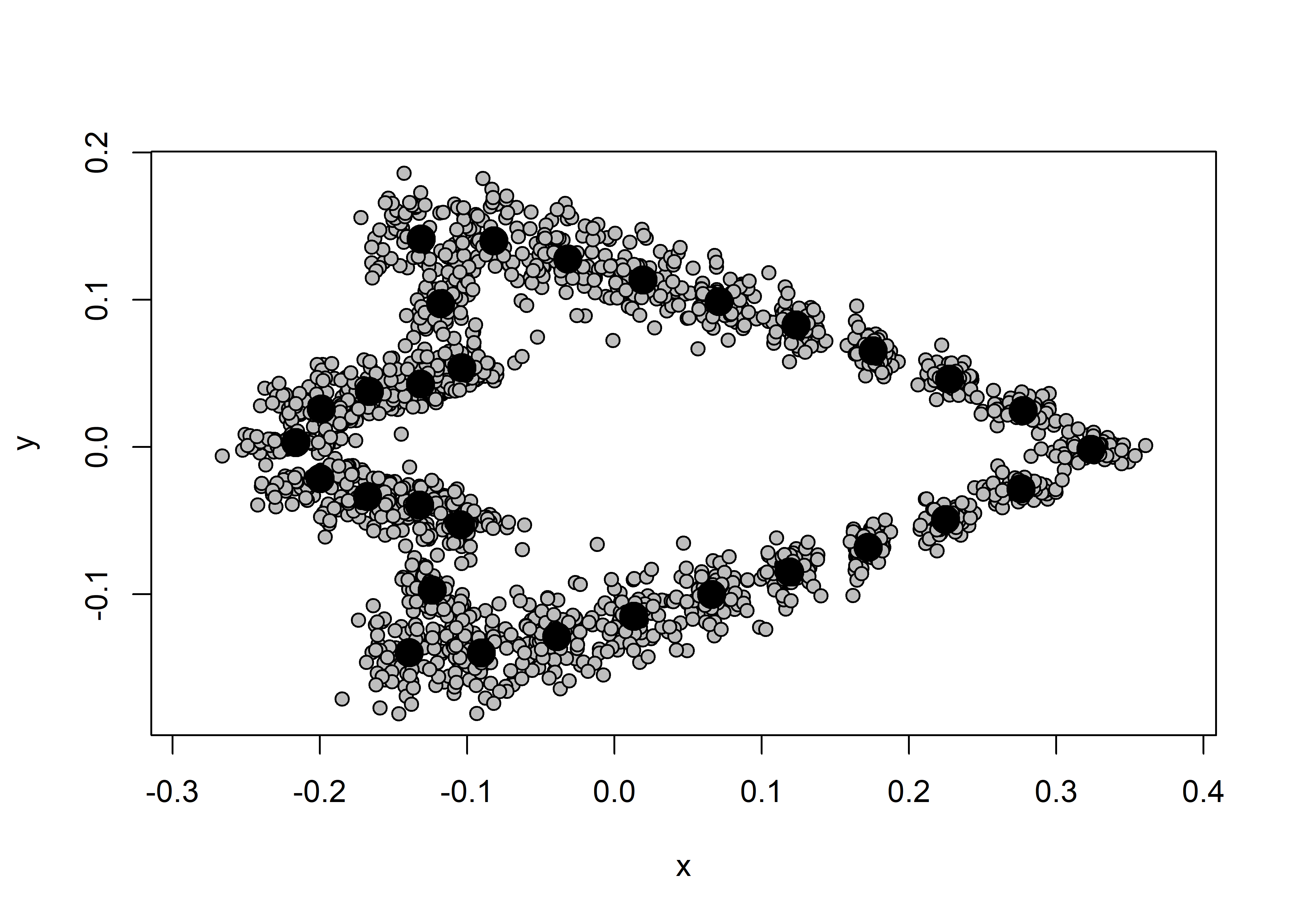
# dataframe
gdf <- geomorph.data.frame(shape = Y.gpa$coords,
                           size = Y.gpa$Csize)
1.3 2BPLS Maximum length
1.3.1 Shape
# is Perdiz arrow point shape correlated with linear var?
shapeml <- two.b.pls(Y.gpa$coords,
                      qdata$maxl,
                      iter = 9999,
                      seed = NULL,
                      print.progress = FALSE)
## Data in either A1 or A2 do not have names. It is assumed data in both A1 and A2 are ordered the same.summary(shapeml)##
## Call:
## two.b.pls(A1 = Y.gpa$coords, A2 = qdata$maxl, iter = 9999, seed = NULL,
## print.progress = FALSE)
##
##
##
## r-PLS: 0.1855
##
## Effect Size (Z): -0.17271
##
## P-value: 0.5668
##
## Based on 10000 random permutations## plot
plot(shapeml)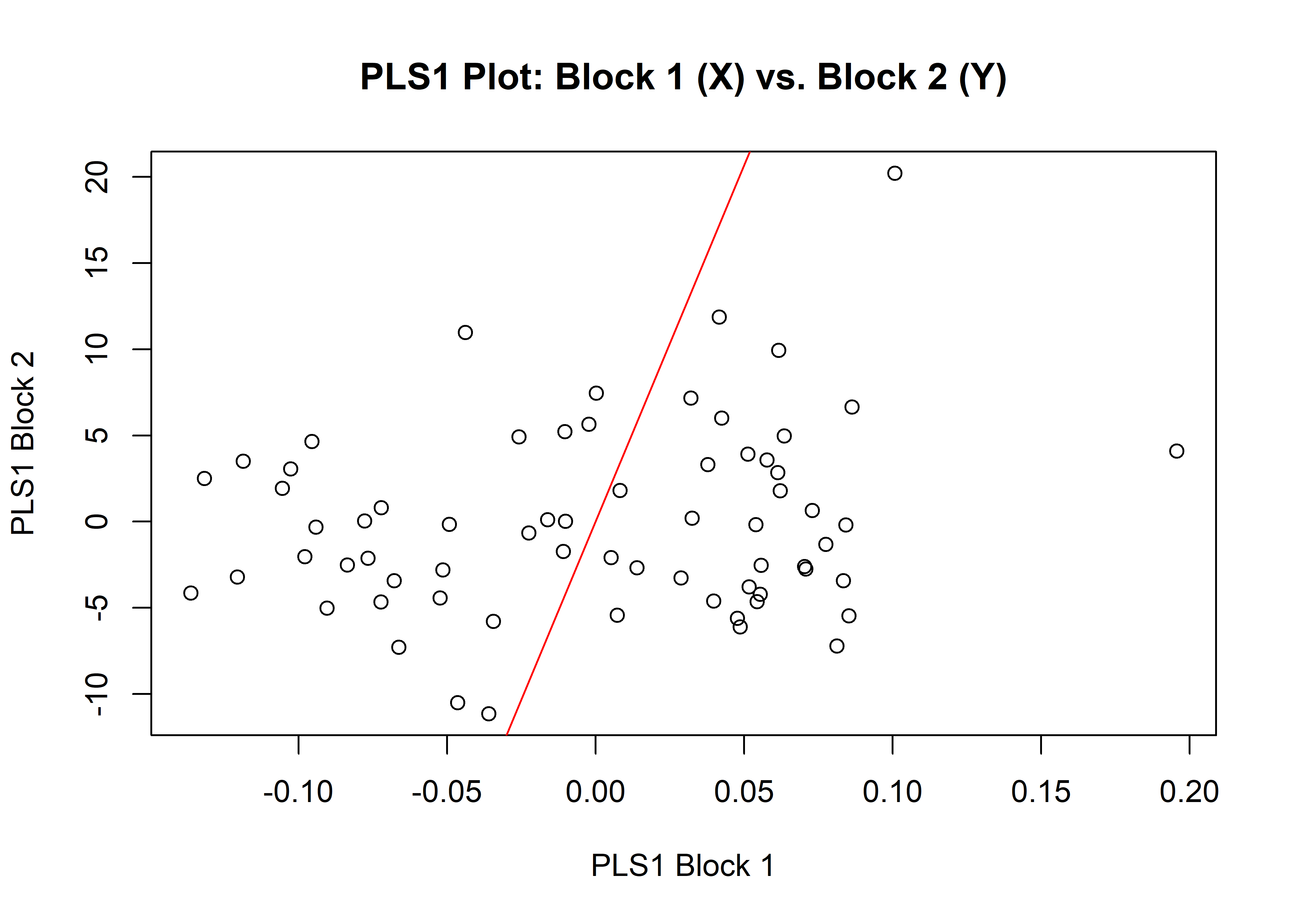
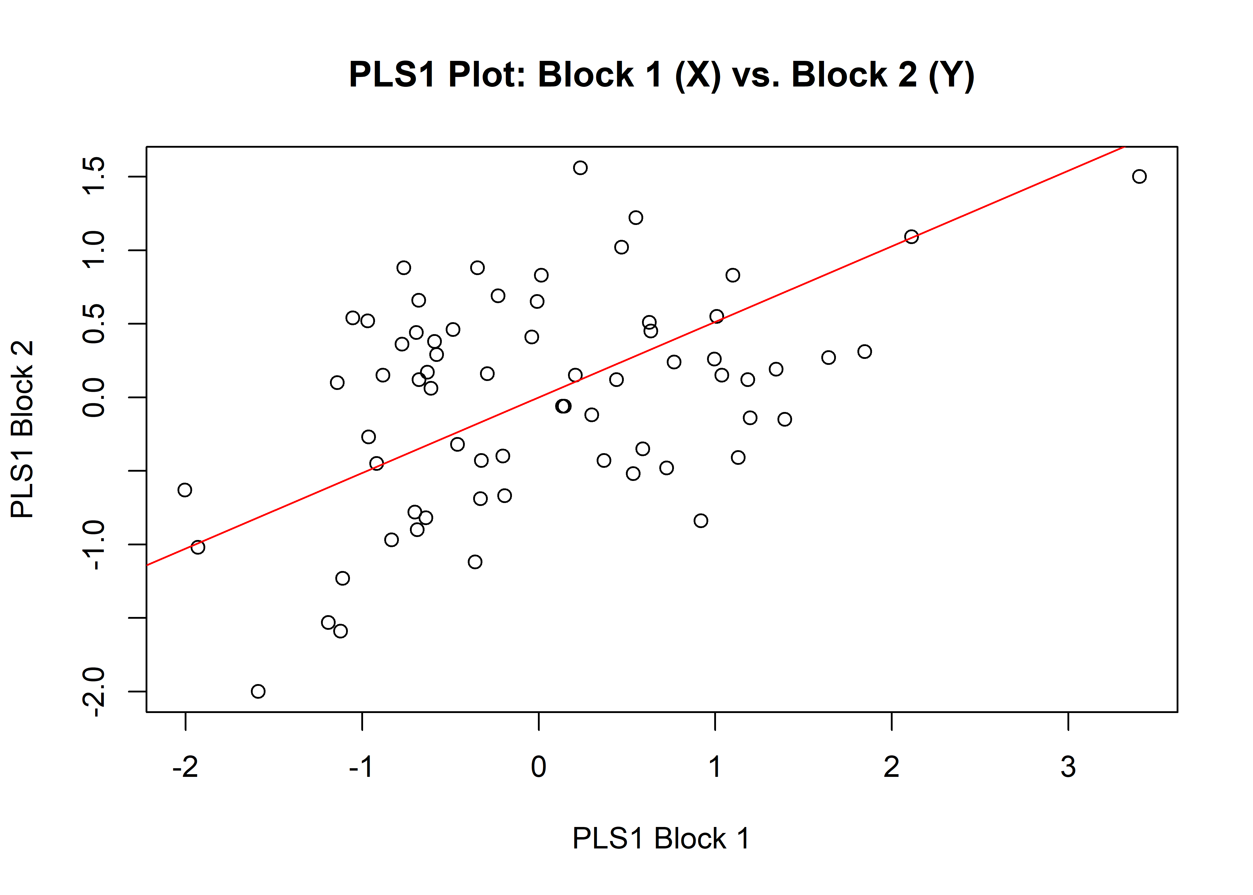
1.3.2 Size
# is Perdiz arrow point size correlated with linear var?
sizeml <- two.b.pls(Y.gpa$Csize,
                      qdata$maxl,
                      iter = 9999,
                      seed = NULL,
                      print.progress = FALSE)
## Data in either A1 or A2 do not have names. It is assumed data in both A1 and A2 are ordered the same.summary(sizeml)##
## Call:
## two.b.pls(A1 = Y.gpa$Csize, A2 = qdata$maxl, iter = 9999, seed = NULL,
## print.progress = FALSE)
##
##
##
## r-PLS: 0.3445
##
## Effect Size (Z): 2.7643
##
## P-value: 0.0041
##
## Based on 10000 random permutations## plot
plot(sizeml)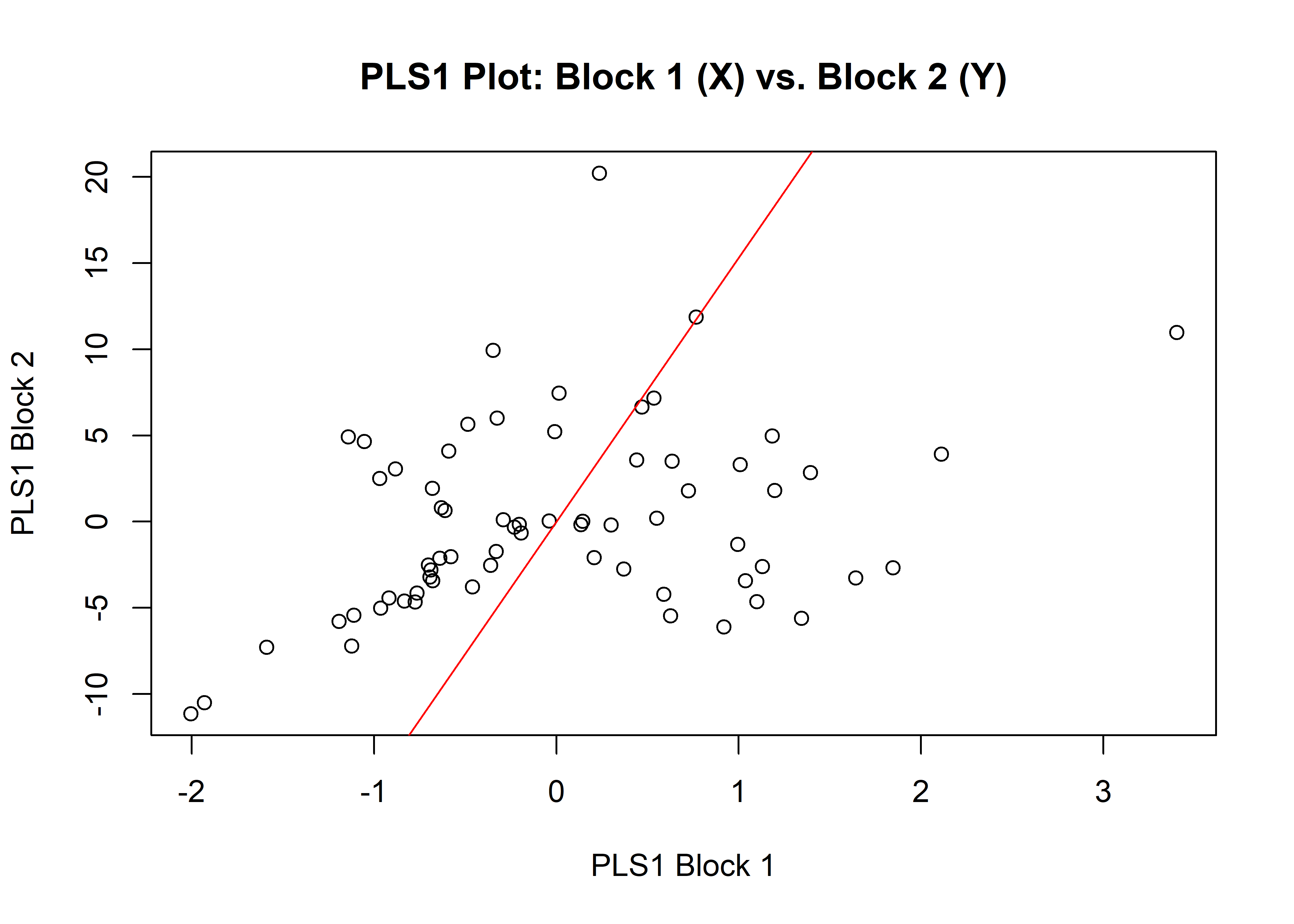
1.4 2BPLS Maximum blade length
1.4.1 Shape
# is Perdiz arrow point shape correlated with linear var?
shapembl <- two.b.pls(Y.gpa$coords,
                      qdata$maxbl,
                      iter = 9999,
                      seed = NULL,
                      print.progress = FALSE)
## Data in either A1 or A2 do not have names. It is assumed data in both A1 and A2 are ordered the same.summary(shapembl)##
## Call:
## two.b.pls(A1 = Y.gpa$coords, A2 = qdata$maxbl, iter = 9999, seed = NULL,
## print.progress = FALSE)
##
##
##
## r-PLS: 0.2858
##
## Effect Size (Z): 1.27424
##
## P-value: 0.1049
##
## Based on 10000 random permutations## plot
plot(shapembl)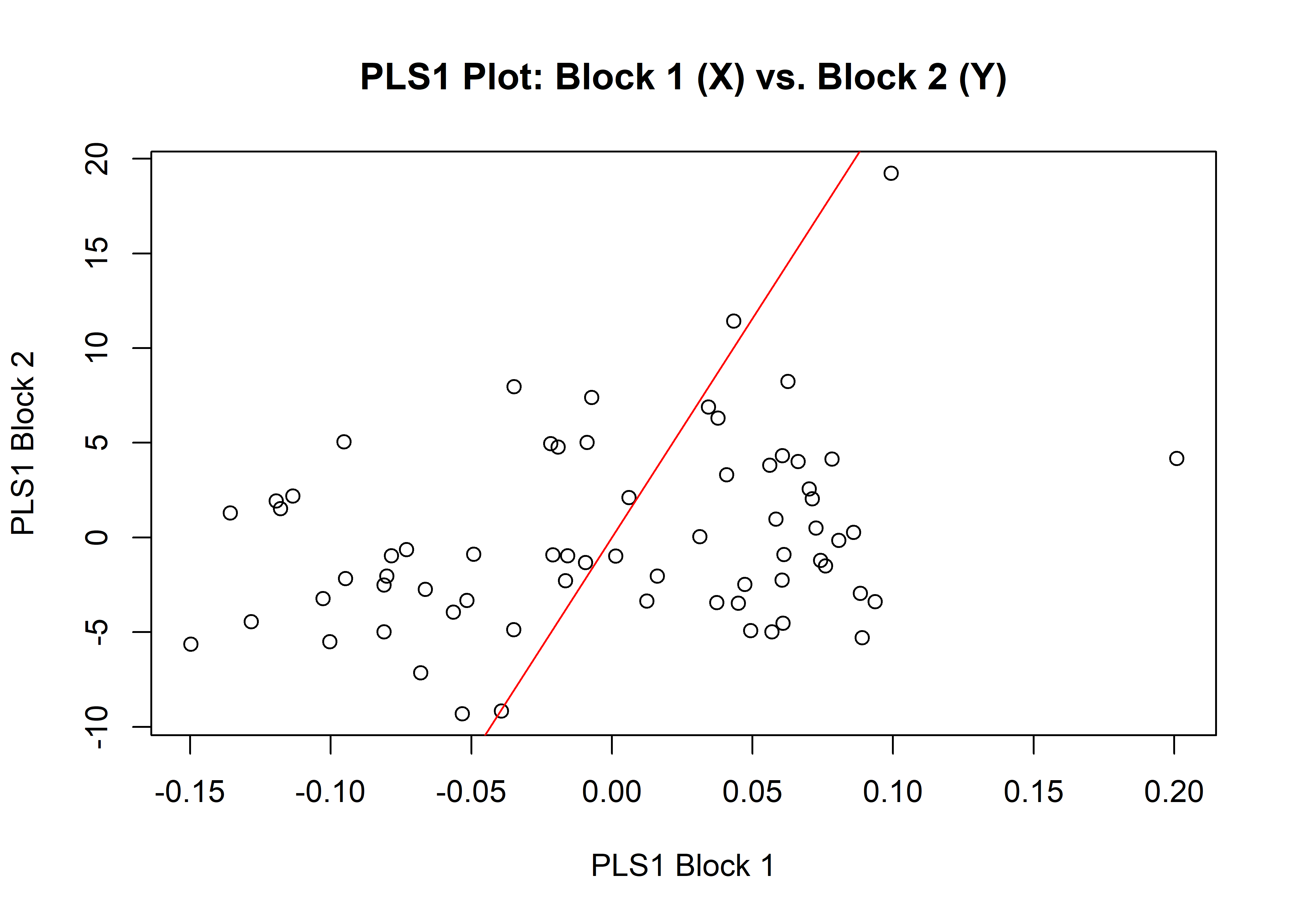
1.4.2 Size
# is Perdiz arrow point size correlated with linear var?
sizembl <- two.b.pls(Y.gpa$Csize,
                      qdata$maxbl,
                      iter = 9999,
                      seed = NULL,
                      print.progress = FALSE)
## Data in either A1 or A2 do not have names. It is assumed data in both A1 and A2 are ordered the same.summary(sizembl)##
## Call:
## two.b.pls(A1 = Y.gpa$Csize, A2 = qdata$maxbl, iter = 9999, seed = NULL,
## print.progress = FALSE)
##
##
##
## r-PLS: 0.3381
##
## Effect Size (Z): 2.69984
##
## P-value: 0.0044
##
## Based on 10000 random permutations## plot
plot(sizembl)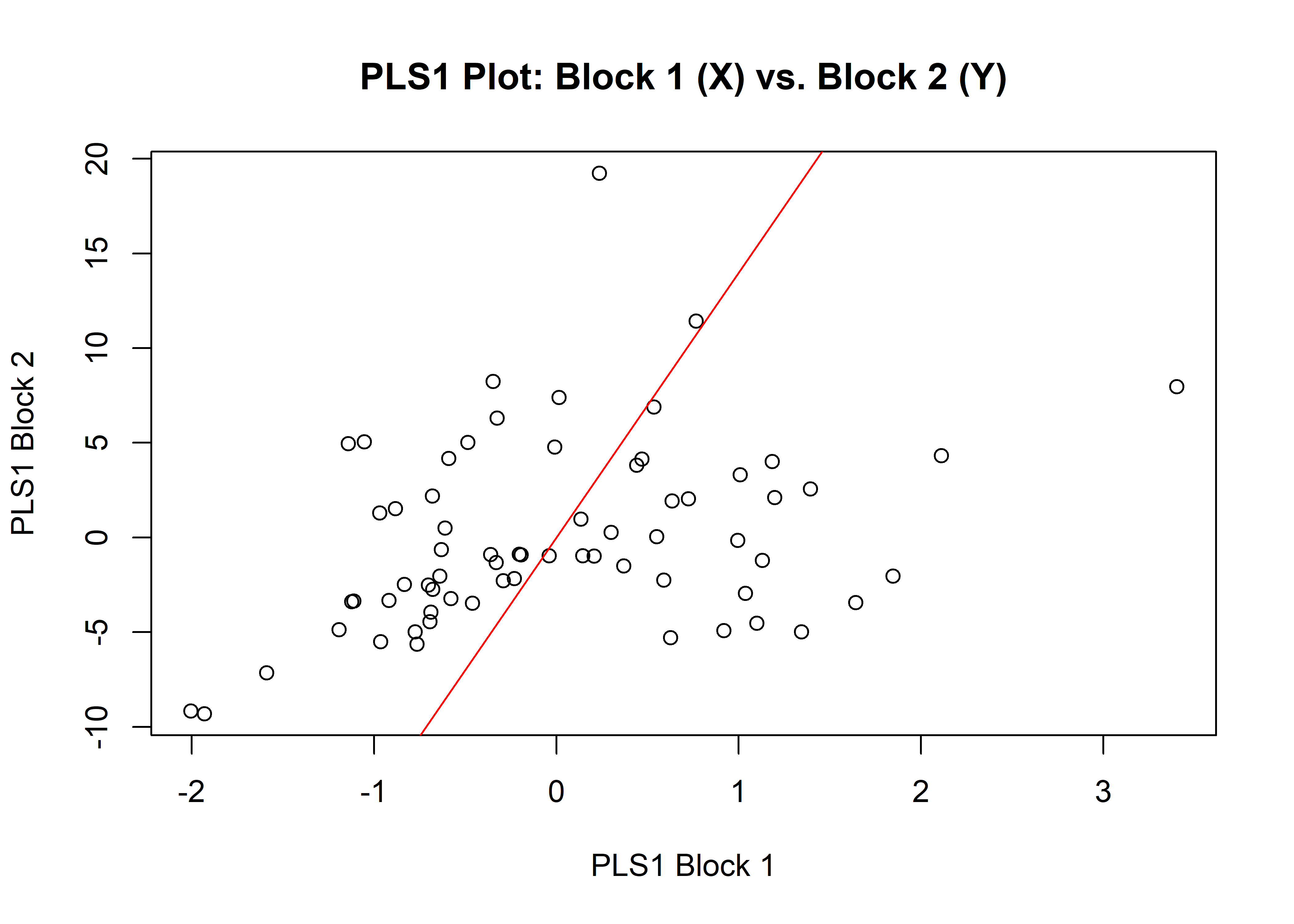
1.5 2BPLS Maximum shoulder width
1.5.1 Shape
# is Perdiz arrow point shape correlated with linear var?
shapemshw <- two.b.pls(Y.gpa$coords,
                      qdata$maxshw,
                      iter = 9999,
                      seed = NULL,
                      print.progress = FALSE)
## Data in either A1 or A2 do not have names. It is assumed data in both A1 and A2 are ordered the same.summary(shapemshw)##
## Call:
## two.b.pls(A1 = Y.gpa$coords, A2 = qdata$maxshw, iter = 9999,
## seed = NULL, print.progress = FALSE)
##
##
##
## r-PLS: 0.3082
##
## Effect Size (Z): 1.49334
##
## P-value: 0.07
##
## Based on 10000 random permutations## plot
plot(shapemshw)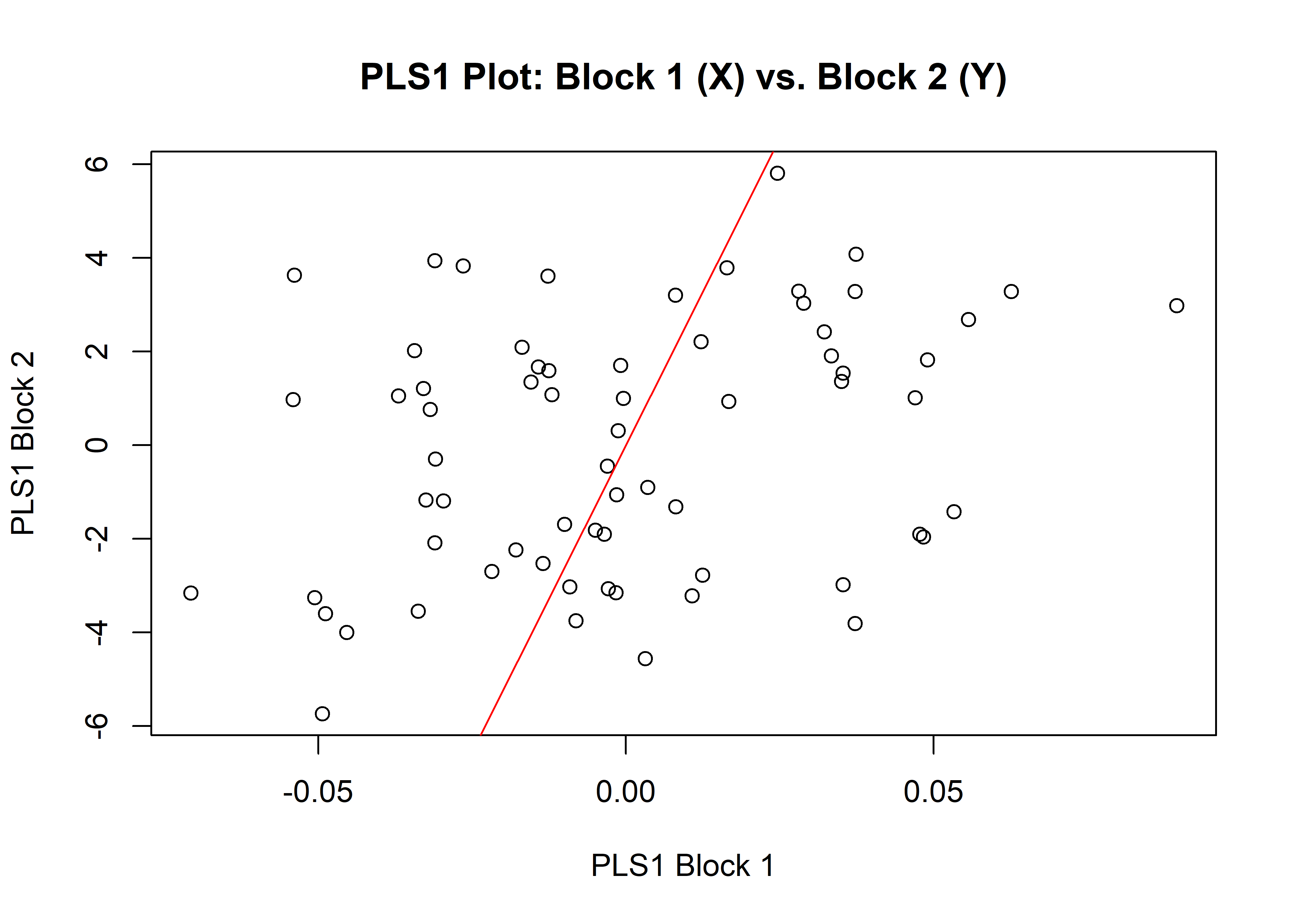
1.5.2 Size
# is Perdiz arrow point size correlated with linear var?
sizemshw <- two.b.pls(Y.gpa$Csize,
                      qdata$maxshw,
                      iter = 9999,
                      seed = NULL,
                      print.progress = FALSE)
## Data in either A1 or A2 do not have names. It is assumed data in both A1 and A2 are ordered the same.summary(sizemshw)##
## Call:
## two.b.pls(A1 = Y.gpa$Csize, A2 = qdata$maxshw, iter = 9999, seed = NULL,
## print.progress = FALSE)
##
##
##
## r-PLS: 0.111
##
## Effect Size (Z): 0.89959
##
## P-value: 0.3712
##
## Based on 10000 random permutations## plot
plot(sizemshw)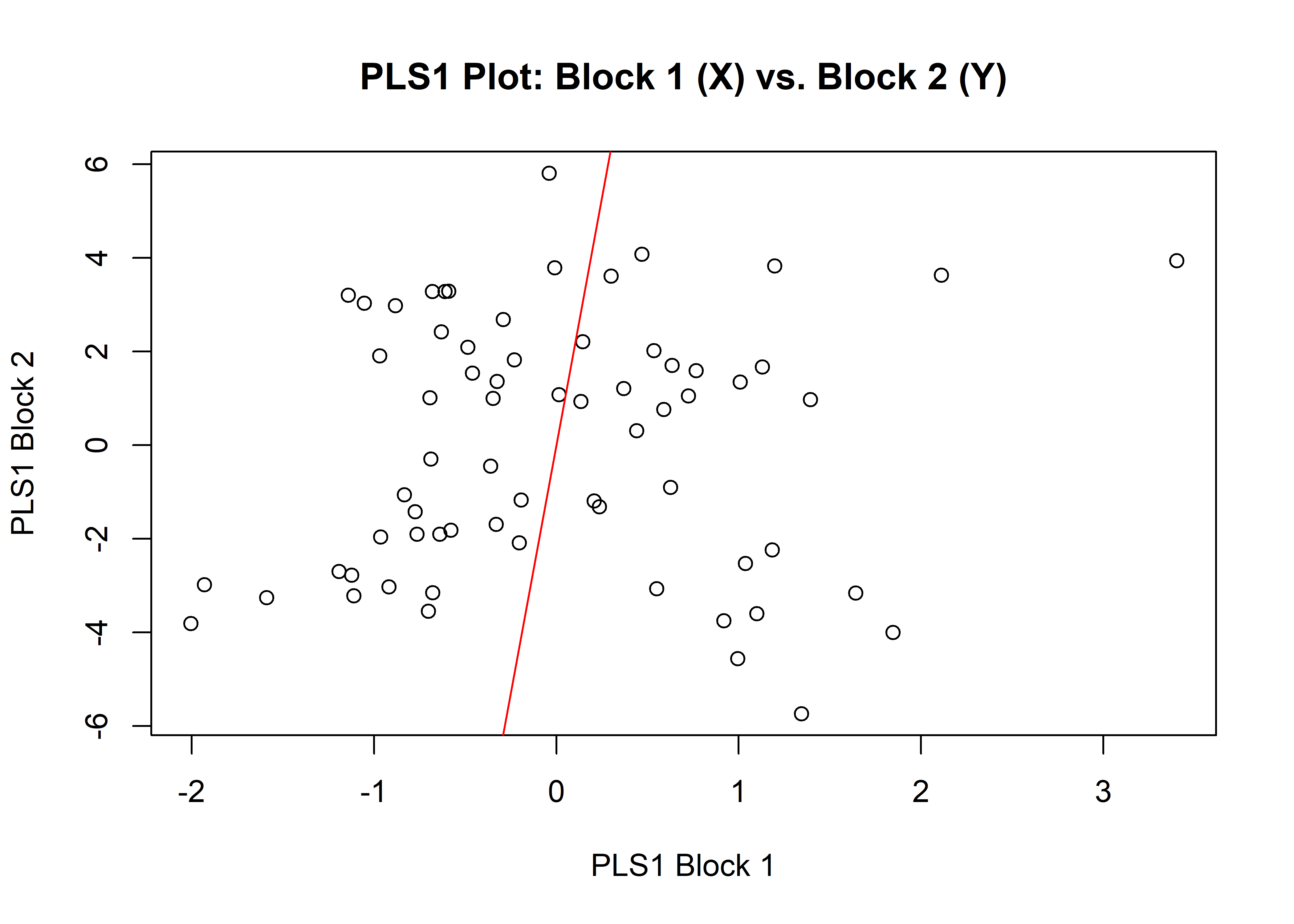
1.6 2BPLS Maximum width
1.6.1 Shape
# is Perdiz arrow point shape correlated with linear var?
shapemw <- two.b.pls(Y.gpa$coords,
                      qdata$maxw,
                      iter = 9999,
                      seed = NULL,
                      print.progress = FALSE)
## Data in either A1 or A2 do not have names. It is assumed data in both A1 and A2 are ordered the same.summary(shapemw)##
## Call:
## two.b.pls(A1 = Y.gpa$coords, A2 = qdata$maxw, iter = 9999, seed = NULL,
## print.progress = FALSE)
##
##
##
## r-PLS: 0.2963
##
## Effect Size (Z): 1.36161
##
## P-value: 0.0923
##
## Based on 10000 random permutations## plot
plot(shapemw)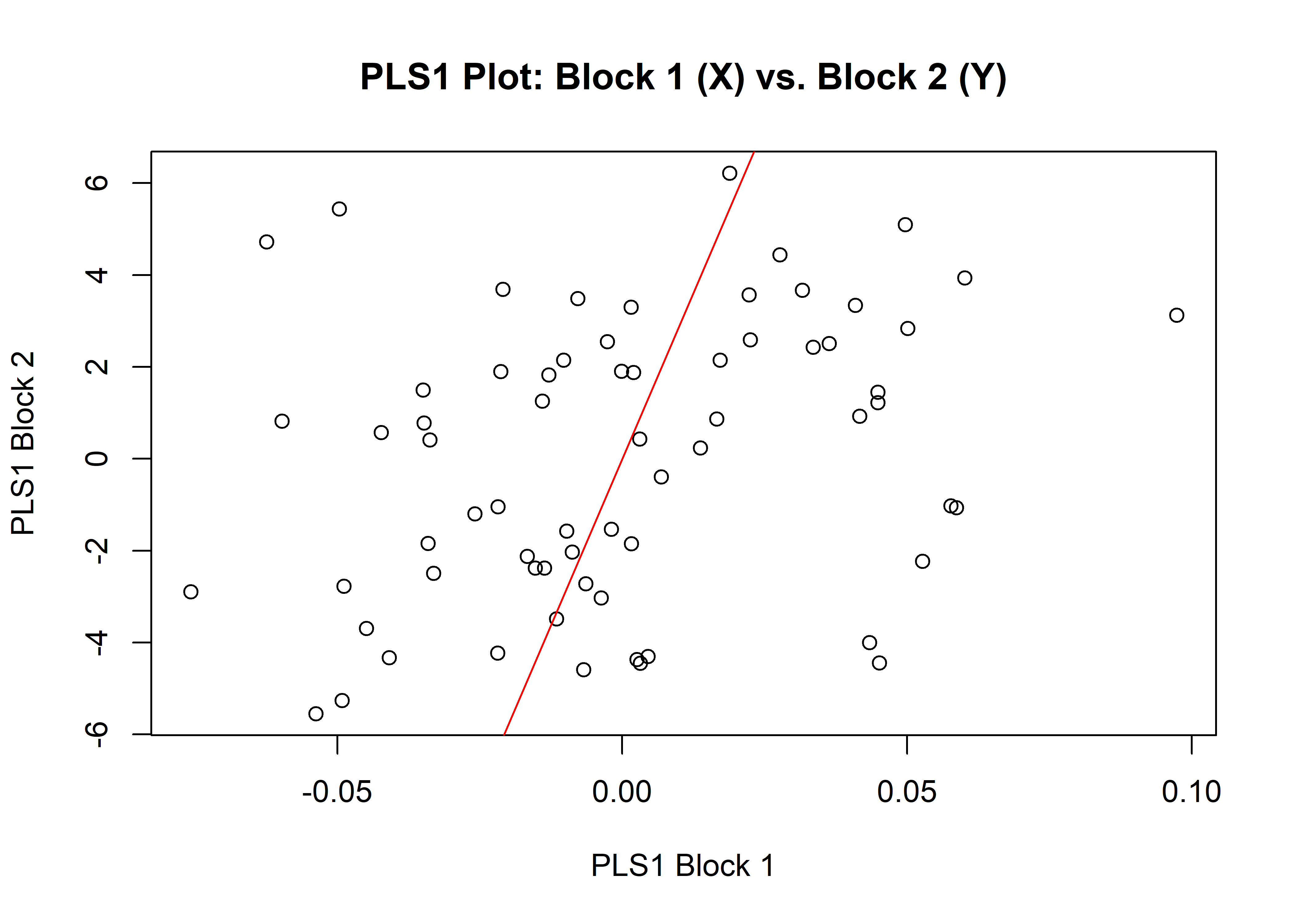
1.6.2 Size
# is Perdiz arrow point size correlated with linear var?
sizemw <- two.b.pls(Y.gpa$Csize,
                      qdata$maxw,
                      iter = 9999,
                      seed = NULL,
                      print.progress = FALSE)
## Data in either A1 or A2 do not have names. It is assumed data in both A1 and A2 are ordered the same.summary(sizemw)##
## Call:
## two.b.pls(A1 = Y.gpa$Csize, A2 = qdata$maxw, iter = 9999, seed = NULL,
## print.progress = FALSE)
##
##
##
## r-PLS: 0.206
##
## Effect Size (Z): 1.67231
##
## P-value: 0.0944
##
## Based on 10000 random permutations## plot
plot(sizemw)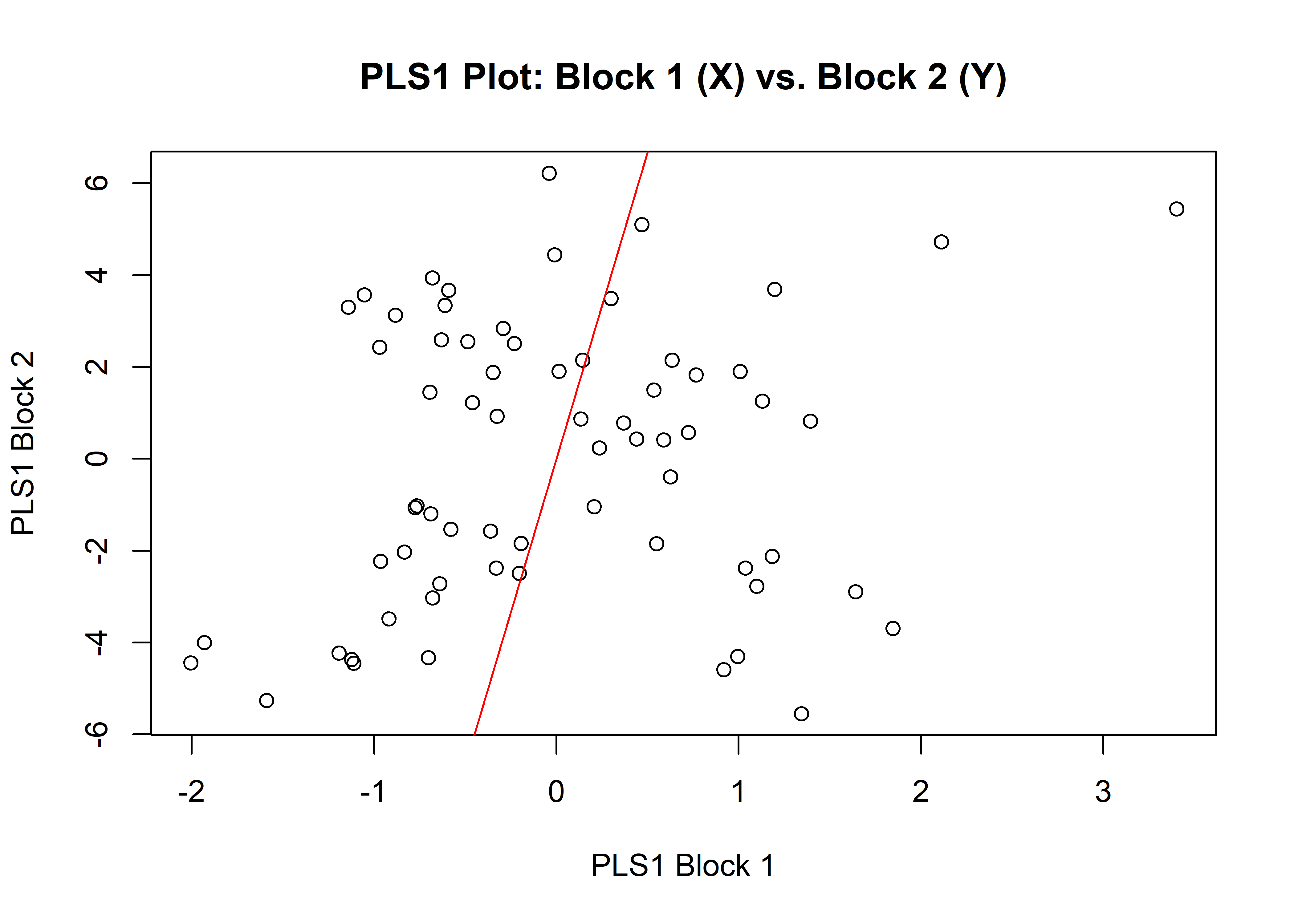
1.7 2BPLS Maximum thickness
1.7.1 Shape
# is Perdiz arrow point shape correlated with linear var?
shapemth <- two.b.pls(Y.gpa$coords,
                      qdata$maxth,
                      iter = 9999,
                      seed = NULL,
                      print.progress = FALSE)
## Data in either A1 or A2 do not have names. It is assumed data in both A1 and A2 are ordered the same.summary(shapemth)##
## Call:
## two.b.pls(A1 = Y.gpa$coords, A2 = qdata$maxth, iter = 9999, seed = NULL,
## print.progress = FALSE)
##
##
##
## r-PLS: 0.2108
##
## Effect Size (Z): 0.2434
##
## P-value: 0.4067
##
## Based on 10000 random permutations## plot
plot(shapemth)
1.7.2 Size
# is Perdiz arrow point size correlated with linear var?
sizemth <- two.b.pls(Y.gpa$Csize,
                      qdata$maxth,
                      iter = 9999,
                      seed = NULL,
                      print.progress = FALSE)
## Data in either A1 or A2 do not have names. It is assumed data in both A1 and A2 are ordered the same.summary(sizemth)##
## Call:
## two.b.pls(A1 = Y.gpa$Csize, A2 = qdata$maxth, iter = 9999, seed = NULL,
## print.progress = FALSE)
##
##
##
## r-PLS: 0.1291
##
## Effect Size (Z): 1.0525
##
## P-value: 0.3059
##
## Based on 10000 random permutations## plot
plot(sizemth)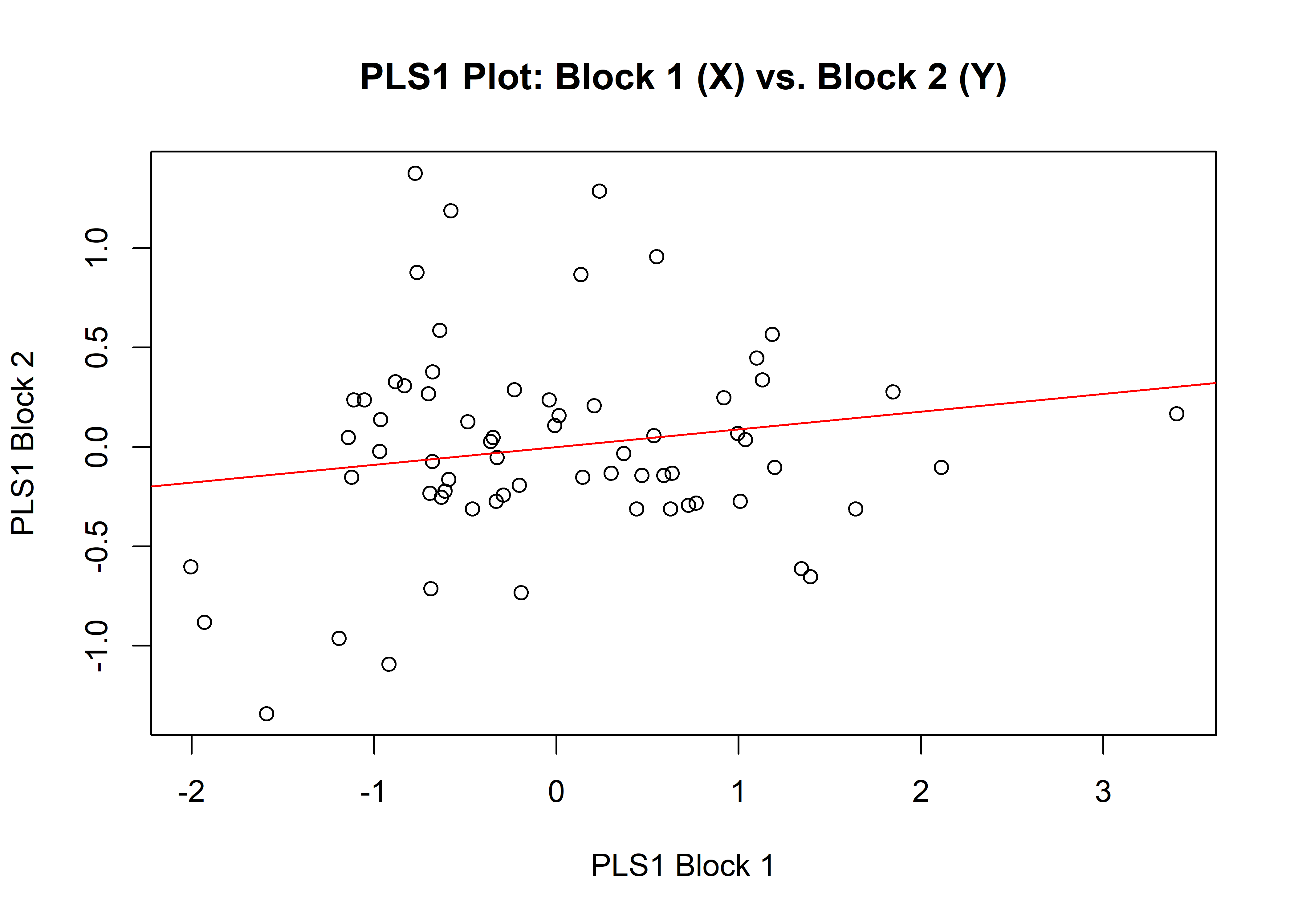
1.8 2BPLS Maximum stem length
1.8.1 Shape
# is Perdiz arrow point shape correlated with linear var?
shapemstl <- two.b.pls(Y.gpa$coords,
                      qdata$maxstl,
                      iter = 9999,
                      seed = NULL,
                      print.progress = FALSE)
## Data in either A1 or A2 do not have names. It is assumed data in both A1 and A2 are ordered the same.summary(shapemstl)##
## Call:
## two.b.pls(A1 = Y.gpa$coords, A2 = qdata$maxstl, iter = 9999,
## seed = NULL, print.progress = FALSE)
##
##
##
## r-PLS: 0.4003
##
## Effect Size (Z): 2.42637
##
## P-value: 0.0052
##
## Based on 10000 random permutations## plot
plot(shapemstl)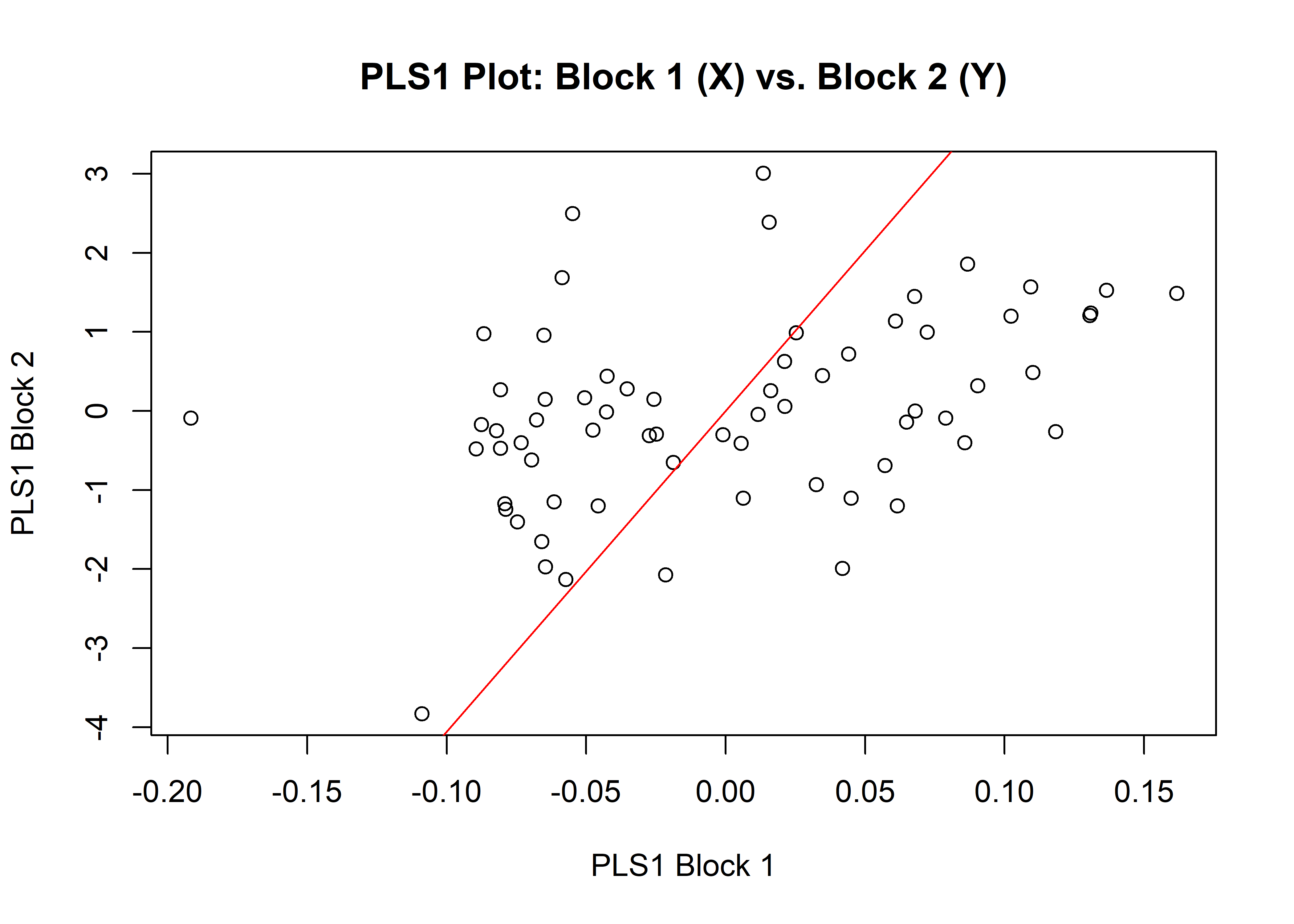
1.8.2 Size
# is Perdiz arrow point size correlated with linear var?
sizemstl <- two.b.pls(Y.gpa$Csize,
                      qdata$maxstl,
                      iter = 9999,
                      seed = NULL,
                      print.progress = FALSE)
## Data in either A1 or A2 do not have names. It is assumed data in both A1 and A2 are ordered the same.summary(sizemstl)##
## Call:
## two.b.pls(A1 = Y.gpa$Csize, A2 = qdata$maxstl, iter = 9999, seed = NULL,
## print.progress = FALSE)
##
##
##
## r-PLS: 0.1762
##
## Effect Size (Z): 1.45327
##
## P-value: 0.1478
##
## Based on 10000 random permutations## plot
plot(sizemstl)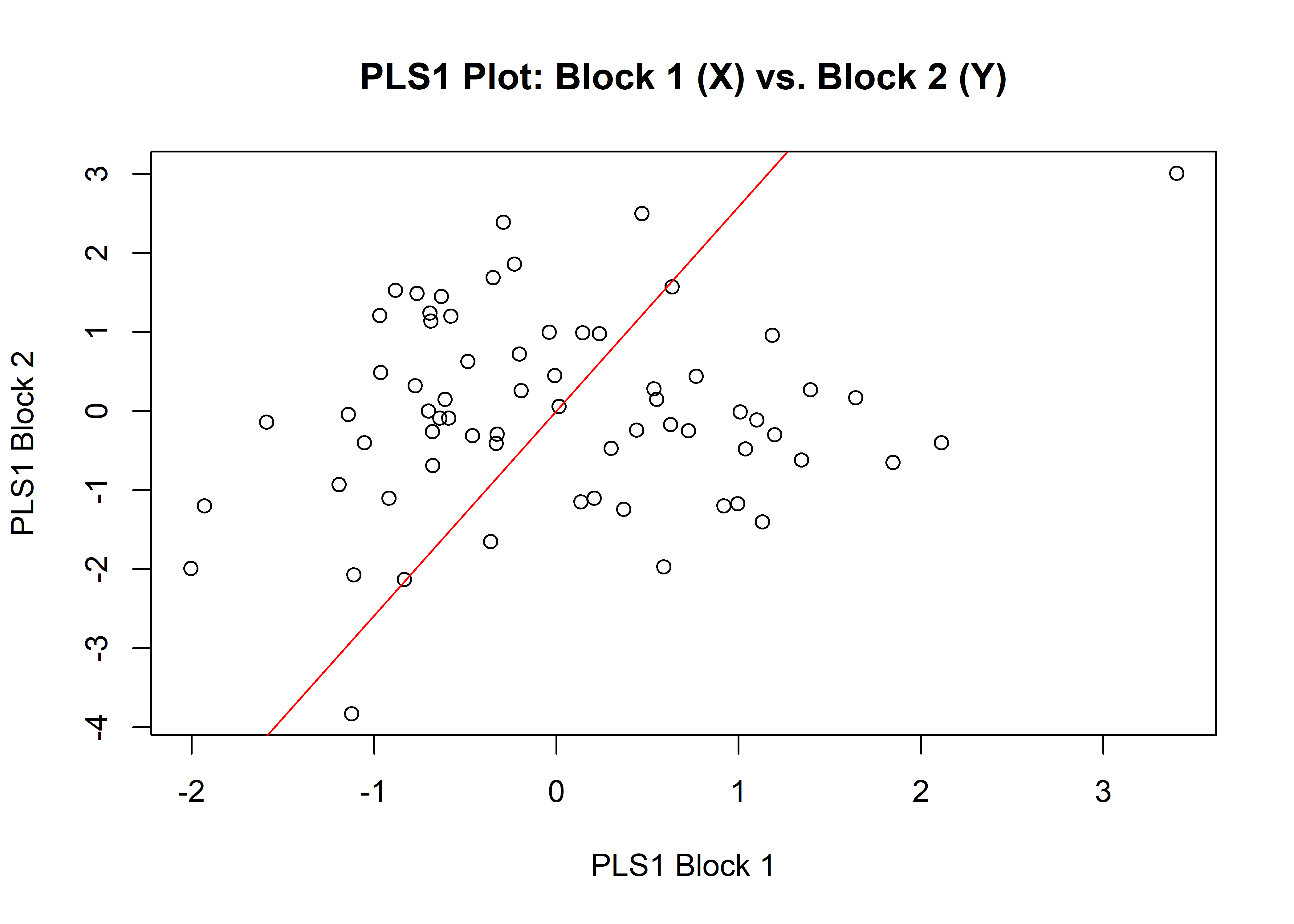
1.9 2BPLS Maximum stem width
1.9.1 Shape
# is Perdiz arrow point shape correlated with linear var?
shapemstw <- two.b.pls(Y.gpa$coords,
                      qdata$maxstw,
                      iter = 9999,
                      seed = NULL,
                      print.progress = FALSE)
## Data in either A1 or A2 do not have names. It is assumed data in both A1 and A2 are ordered the same.summary(shapemstw)##
## Call:
## two.b.pls(A1 = Y.gpa$coords, A2 = qdata$maxstw, iter = 9999,
## seed = NULL, print.progress = FALSE)
##
##
##
## r-PLS: 0.1585
##
## Effect Size (Z): -0.64787
##
## P-value: 0.7304
##
## Based on 10000 random permutations## plot
plot(shapemstw)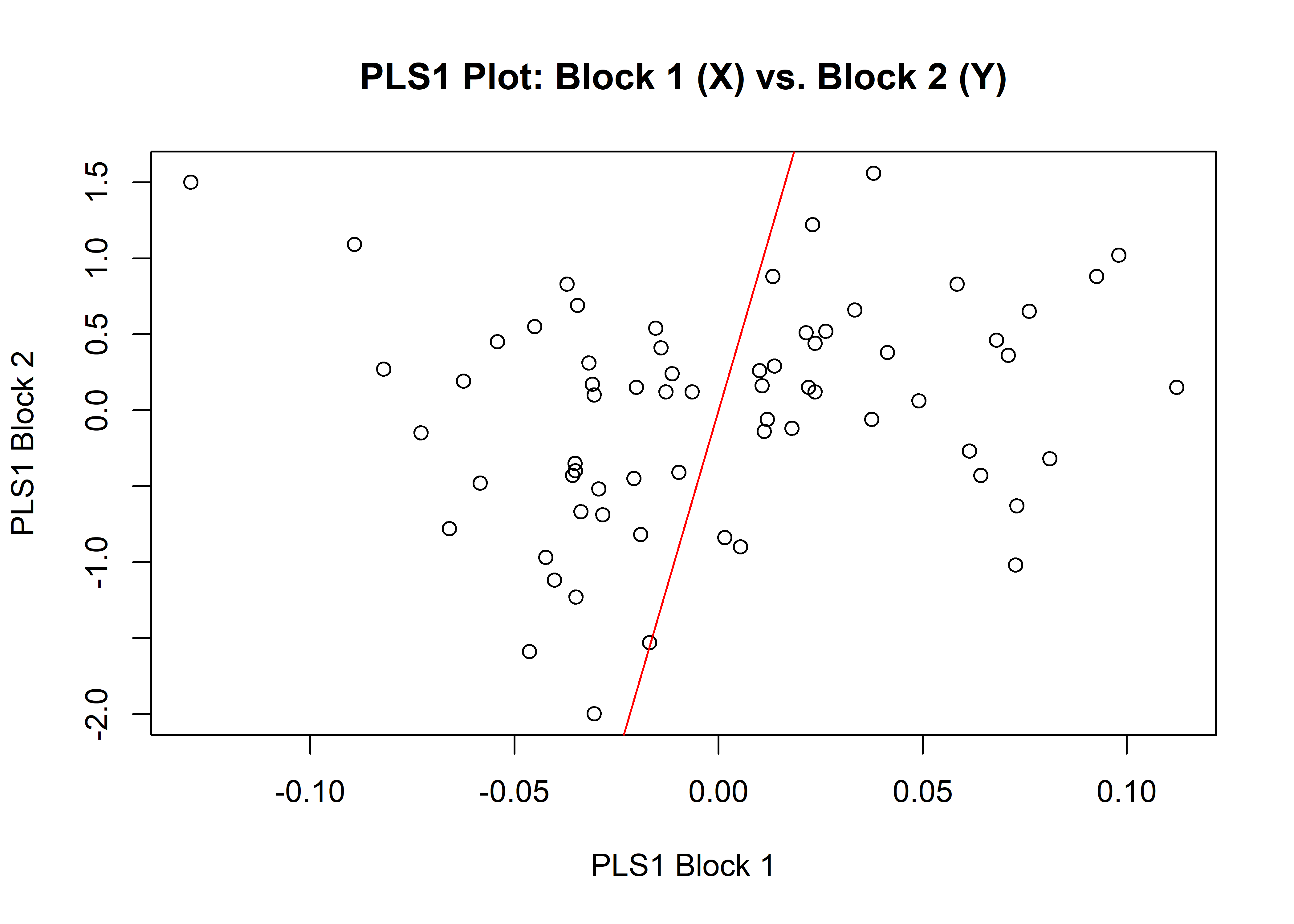
1.9.2 Size
# is Perdiz arrow point size correlated with linear var?
sizemstw <- two.b.pls(Y.gpa$Csize,
                      qdata$maxstw,
                      iter = 9999,
                      seed = NULL,
                      print.progress = FALSE)
## Data in either A1 or A2 do not have names. It is assumed data in both A1 and A2 are ordered the same.summary(sizemstw)##
## Call:
## two.b.pls(A1 = Y.gpa$Csize, A2 = qdata$maxstw, iter = 9999, seed = NULL,
## print.progress = FALSE)
##
##
##
## r-PLS: 0.4524
##
## Effect Size (Z): 3.67031
##
## P-value: 2e-04
##
## Based on 10000 random permutations## plot
plot(sizemstw)