Geometric Morphometrics

Does elliptical biface morphology differ between ColorGroup A and ColorGroup B?

Load packages + data

# load required analysis packages
library(here)
here() starts at /Users/seldenjrz/Documents/github/elliptical.bifaces.1/supp
library(StereoMorph)
library(geomorph)
Loading required package: RRPP
Loading required package: rgl
Loading required package: Matrix
library(tidyverse)
── Attaching core tidyverse packages ──────────────────────── tidyverse 2.0.0 ──
✔ dplyr     1.1.2     ✔ readr     2.1.4
✔ forcats   1.0.0     ✔ stringr   1.5.0
✔ ggplot2   3.4.2     ✔ tibble    3.2.1
✔ lubridate 1.9.2     ✔ tidyr     1.3.0
✔ purrr     1.0.1     
── Conflicts ────────────────────────────────────────── tidyverse_conflicts() ──
✖ tidyr::expand() masks Matrix::expand()
✖ dplyr::filter() masks stats::filter()
✖ dplyr::lag()    masks stats::lag()
✖ tidyr::pack()   masks Matrix::pack()
✖ tidyr::unpack() masks Matrix::unpack()
ℹ Use the conflicted package (<http://conflicted.r-lib.org/>) to force all conflicts to become errors
library(wesanderson)
library(ggplot2)

# read data and define number of sLMs ----
shapes <- readShapes("shapes")
shapesGM <- readland.shapes(shapes, nCurvePts = c(15, 20, 35))

# read categorical data
qdata <- read.csv("qdata2.csv", 
                  header = TRUE, 
                  row.names = 1)

Generalised Procrustes Analysis

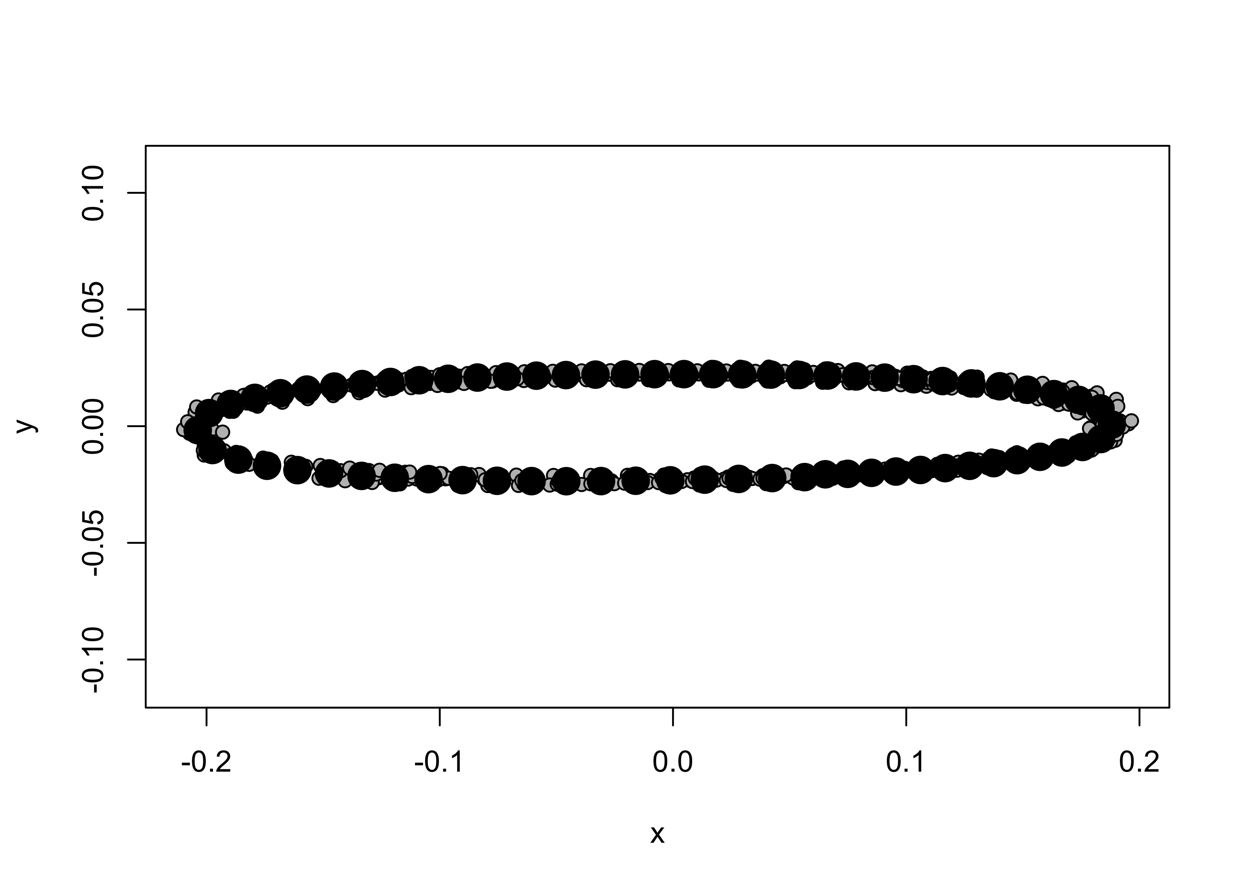
Landmark data were aligned to a global coordinate system (Kendall 1981, 1984; Slice 2001), achieved through generalized Procrustes superimposition (Rohlf and Slice 1990) performed in R (R Core Development Team, 2023) using the geomorph library (Adams et al. 2017; Adams and Otarola-Castillo 2013; Baken et al. 2021). Procrustes superimposition translates, scales, and rotates the coordinate data to allow for comparisons among objects (Gower 1975; Rohlf and Slice 1990). The geomorph package uses a partial Procrustes superimposition that projects the aligned specimens into tangent space subsequent to alignment in preparation for the use of multivariate methods that assume linear space (Rohlf 1999; Slice 2001).

# gpa ----
Y.gpa <- gpagen(shapesGM, print.progress = FALSE)

# plot
plot(Y.gpa)

# geomorph data frame ----
gdf <- geomorph.data.frame(shape = Y.gpa$coords, 
                           size = Y.gpa$Csize,
                           ColorGroup = qdata$ColorGroup)

# add centroid size to qdata
qdata$csz <- Y.gpa$Csize

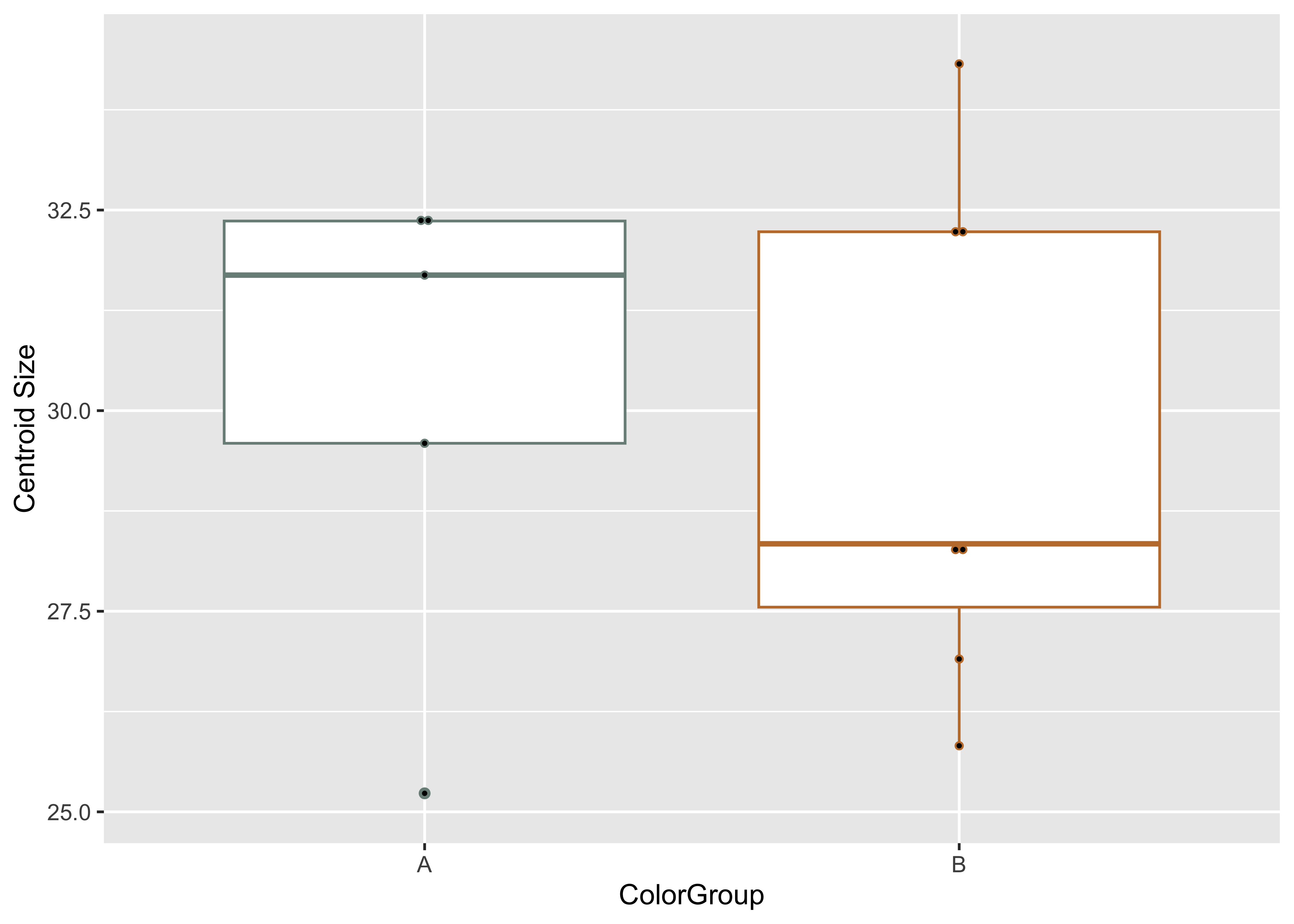
Boxplot (centroid size)

# attributes
csz <- qdata$csz
ColorG <- qdata$ColorGroup

# palette
pal = wes_palette("Moonrise2")

# boxplot of Perdiz arrow points by region
ggplot(qdata, aes(x = ColorG, y = csz, color = ColorG)) +
  geom_boxplot() +
  geom_dotplot(binaxis = 'y', stackdir = 'center', dotsize = 0.3) +
  scale_color_manual(values = pal) +
  theme(legend.position = "none") +
  labs(x = 'ColorGroup', y = 'Centroid Size')
Bin width defaults to 1/30 of the range of the data. Pick better value with
`binwidth`.

Principal Components Analysis

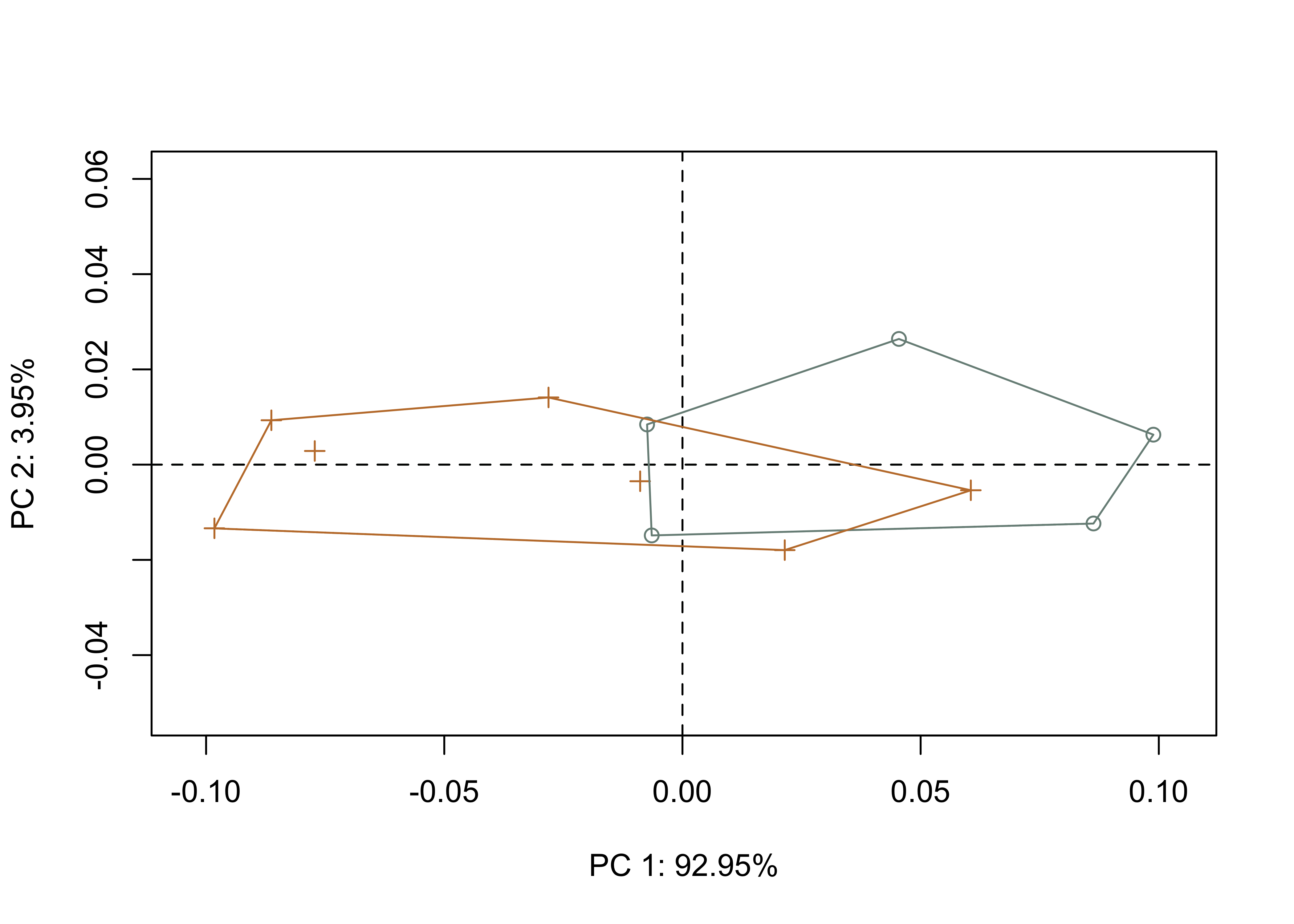
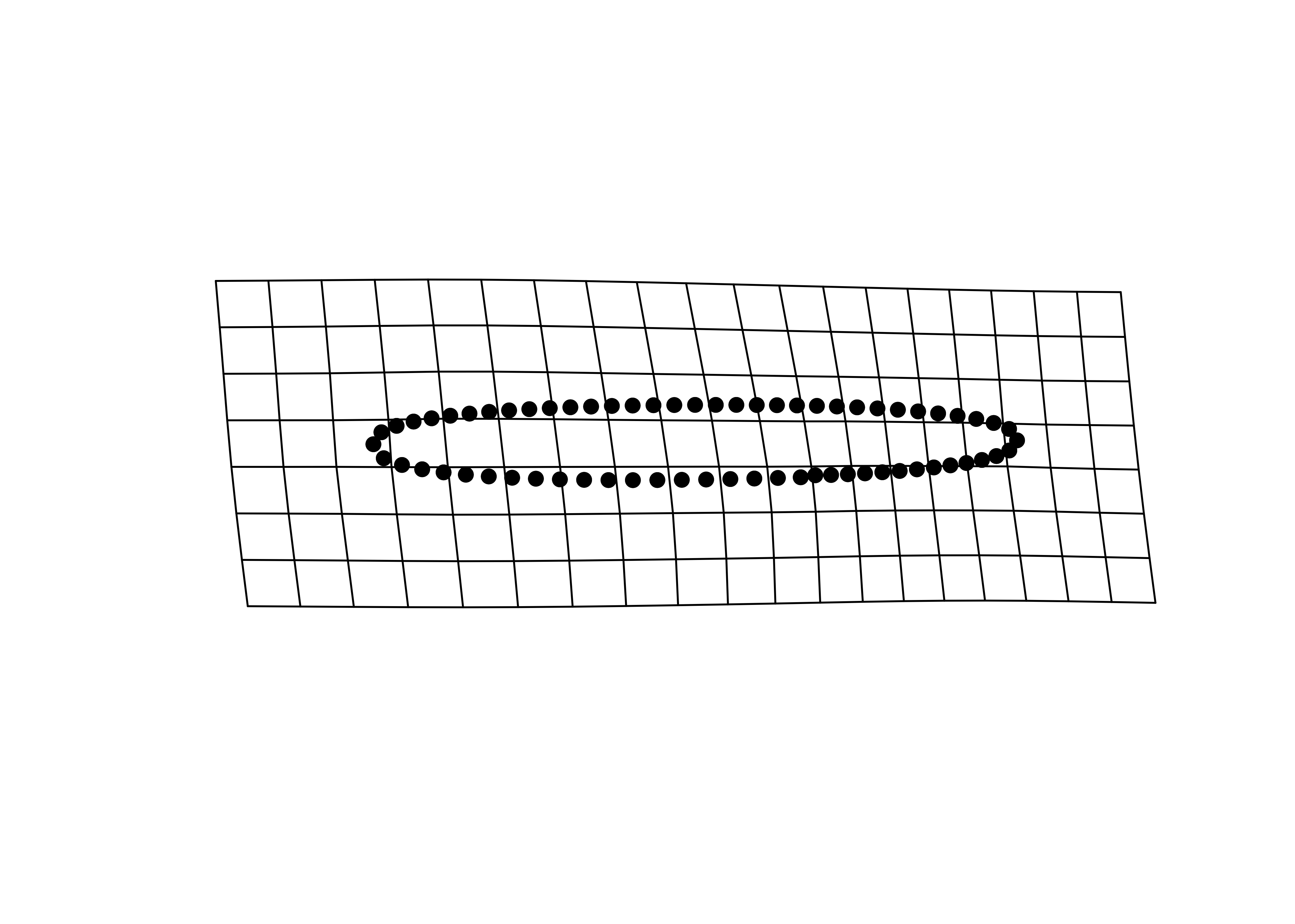
Principal components analysis (Jolliffe 2002) was used to visualise shape variation among the Perdiz arrow points. The shape changes described by each principal axis are commonly visualized using thin-plate spline warping of a reference 3D mesh (Klingenberg 2013; Sherratt et al. 2014).

# principal components analysis ----
pca<-gm.prcomp(Y.gpa$coords)
summary(pca)

Ordination type: Principal Component Analysis 
Centering by OLS mean
Orthogonal projection of OLS residuals
Number of observations: 12 
Number of vectors 11 

Importance of Components:
                             Comp1        Comp2        Comp3        Comp4
Eigenvalues            0.004312448 0.0001834059 8.306817e-05 2.967309e-05
Proportion of Variance 0.929457488 0.0395292921 1.790360e-02 6.395411e-03
Cumulative Proportion  0.929457488 0.9689867800 9.868904e-01 9.932858e-01
                              Comp5        Comp6        Comp7        Comp8
Eigenvalues            1.571728e-05 5.681172e-06 4.247943e-06 2.732388e-06
Proportion of Variance 3.387528e-03 1.224457e-03 9.155547e-04 5.889088e-04
Cumulative Proportion  9.966733e-01 9.978978e-01 9.988133e-01 9.994022e-01
                              Comp9       Comp10       Comp11
Eigenvalues            1.331265e-06 8.238736e-07 6.183380e-07
Proportion of Variance 2.869262e-04 1.775686e-04 1.332697e-04
Cumulative Proportion  9.996892e-01 9.998667e-01 1.000000e+00
# set plot parameters
pch.gps <- c(1,3)[as.factor(qdata$ColorGroup)]
col.gps <- wes_palette("Moonrise2")[as.factor(qdata$ColorGroup)]
col.hull <- c("#798E87","#C27D38")

# plot pca by merged
pc.plot <- plot(pca, 
                asp = 1,
                pch = pch.gps,
                col = col.gps)
shapeHulls(pc.plot, 
           groups = qdata$ColorGroup,
           group.cols = col.hull)

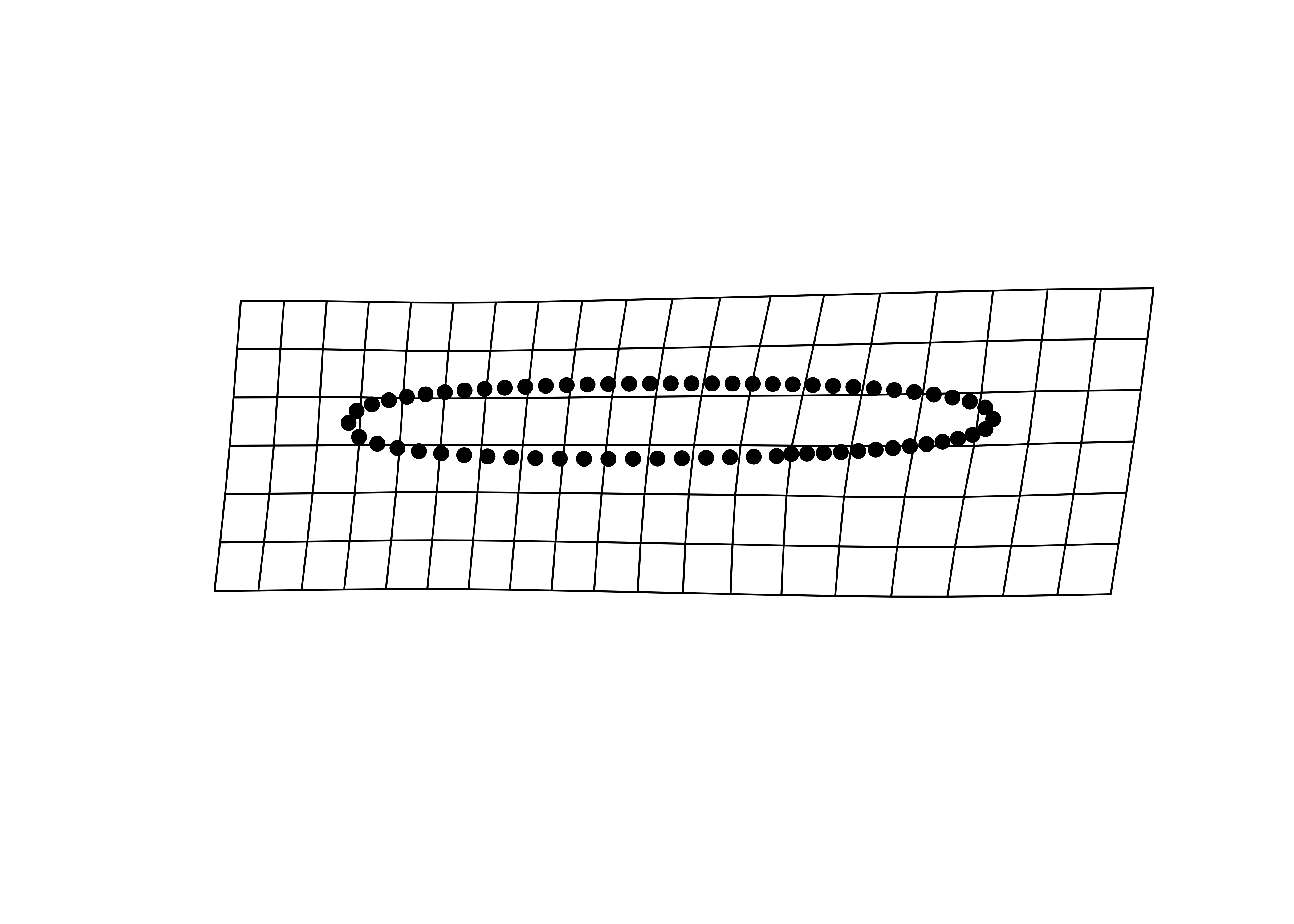
# plot x/y maxima/minima
## x - minima
mean.shape <- mshape(Y.gpa$coords)
plotRefToTarget(pca$shapes$shapes.comp1$min, 
                mean.shape)

## x - maxima
plotRefToTarget(pca$shapes$shapes.comp1$max, 
                mean.shape)

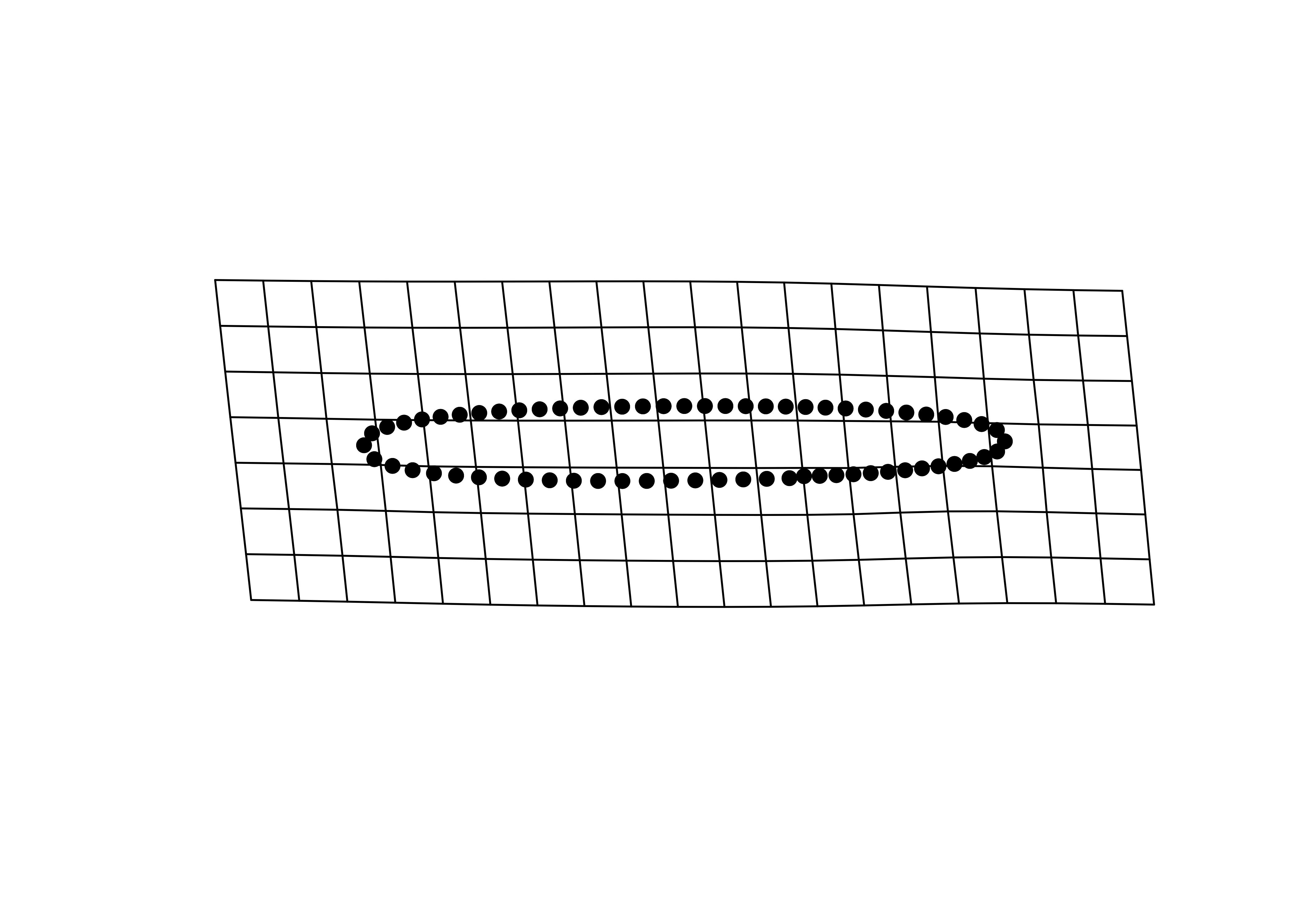
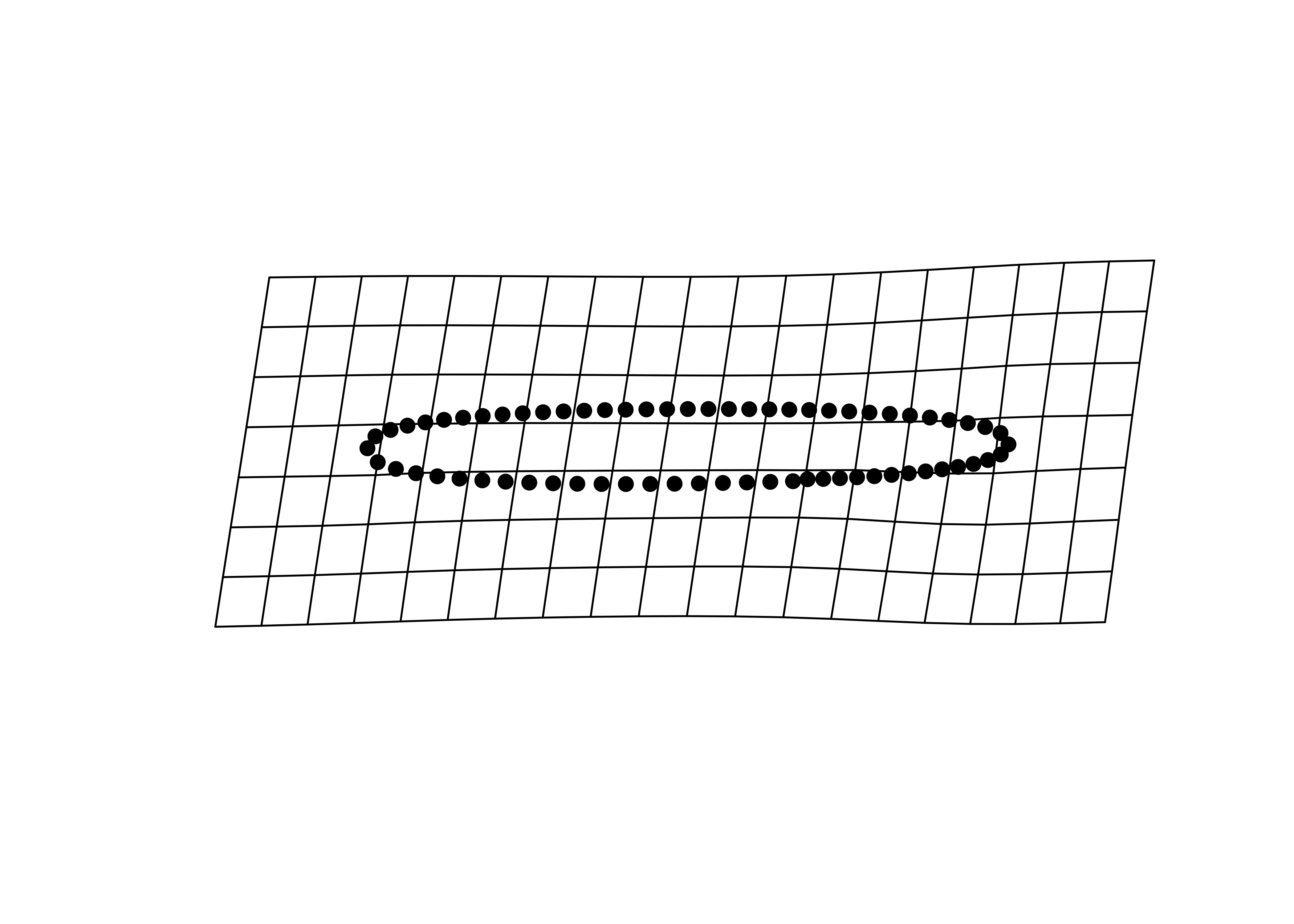
## y - minima
plotRefToTarget(pca$shapes$shapes.comp2$min, 
                mean.shape)

## y - maxima
plotRefToTarget(pca$shapes$shapes.comp2$max, 
                mean.shape)

Procrustes ANOVA

To assess whether shape and size differ by ColorGroup, Procrustes ANOVAs (Goodall 1991) were run that enlist effect-sizes (zscores) computed as standard deviates of the generated sampling distributions (Collyer, Sekora, and Adams 2015). A residual randomization permutation procedure (RRPP; n = 10,000 permutations) was used for all Procrustes ANOVAs (Adams and Collyer 2015; Collyer and Adams 2018), which has higher statistical power and a greater ability to identify patterns in the data should they be present (Anderson and Ter Braak 2003).

# ANOVA ----
# shape
fit.sh <- procD.lm(shape ~ ColorGroup,
                   data = gdf,
                   print.progress = FALSE,
                   iter = 9999)

# shape as a function of ColorGroup/raw material?
anova(fit.sh)

Analysis of Variance, using Residual Randomization
Permutation procedure: Randomization of null model residuals 
Number of permutations: 10000 
Estimation method: Ordinary Least Squares 
Sums of Squares and Cross-products: Type I 
Effect sizes (Z) based on F distributions

           Df       SS        MS     Rsq      F      Z  Pr(>F)  
ColorGroup  1 0.016235 0.0162353 0.31811 4.6651 1.6088 0.04695 *
Residuals  10 0.034802 0.0034802 0.68189                        
Total      11 0.051037                                          
---
Signif. codes:  0 '***' 0.001 '**' 0.01 '*' 0.05 '.' 0.1 ' ' 1

Call: procD.lm(f1 = shape ~ ColorGroup, iter = 9999, data = gdf, print.progress = FALSE)
# size
fit.sz <- procD.lm(size ~ ColorGroup,
                   data = gdf,
                   print.progress = FALSE,
                   iter = 9999)

# size as a function of ColorGroup/raw material?
anova(fit.sz)

Analysis of Variance, using Residual Randomization
Permutation procedure: Randomization of null model residuals 
Number of permutations: 10000 
Estimation method: Ordinary Least Squares 
Sums of Squares and Cross-products: Type I 
Effect sizes (Z) based on F distributions

           Df     SS     MS     Rsq      F        Z Pr(>F)
ColorGroup  1  0.819 0.8190 0.00831 0.0837 -0.74984 0.7803
Residuals  10 97.796 9.7796 0.99169                       
Total      11 98.615                                      

Call: procD.lm(f1 = size ~ ColorGroup, iter = 9999, data = gdf, print.progress = FALSE)

References

Adams, Dean C., and Michael L. Collyer. 2015. Permutation Tests for Phylogenetic Comparative Analyses of High-Dimensional Shape Data: What you Shuffle Matters.” Evolution 69 (3): 823–29. https://doi.org/10.1111/evo.12596.
Adams, Dean C., Michael L. Collyer, Antigoni Kaliontzopoulou, and Emma Sherratt. 2017. Package geomorph: Geometric Morphometric Analyses of Landmark Data. R package version 3.0.5.” http://geomorphr.github.io/geomorph/.
Adams, Dean C., and Erik Otarola-Castillo. 2013. geomorph: An R Package for the Collection and Analysis of Geometric Morphometric Shape Data.” Methods in Ecology and Evolution 4 (4): 393–99. https://doi.org/10.1111/2041-210x.12035.
Anderson, M. J., and C. J. F. Ter Braak. 2003. Permutation Tests for Multi-Factoral Analysis of Variance.” Journal of Statistical Computation and Simulation 73 (2): 85–113. https://doi.org/10.1080=0094965021000015558.
Baken, Erica K., Michael L. Collyer, Antigoni Kaliontzopoulou, and Dean C. Adams. 2021. geomorph v4.0 and gmShiny: Enhanced analytics and a new graphical interface for a comprehensive morphometric experience.” Journal Article. Methods in Ecology and Evolution. https://doi.org/10.1111/2041-210x.13723.
Collyer, Michael L., and Dean C. Adams. 2018. RRPP: An R Package for Fitting Linear Models to High-Dimensional Data using Residual Randomization.” Methods in Ecology and Evolution 9 (7): 1772–79. https://doi.org/https://doi.org/10.1111/2041-210X.13029.
Collyer, Michael L., David J. Sekora, and Dean C. Adams. 2015. A Method for Analysis of Phenotypic Change for Phenotypes Described by High-Dimensional Data.” Heredity 115 (4): 357–65. https://doi.org/10.1038/hdy.2014.75.
Goodall, Colin. 1991. Procrustes Methods in the Statistical Analysis of Shape.” Journal of the Royal Statistical Society. Series B (Methodological) 53 (2): 285–339.
Gower, J. C. 1975. Generalized Procrustes Analysis.” Psychometrika 40 (1): 33–51. https://doi.org/https://doi.org/10.1007/BF02291478.
Jolliffe, Ian T. 2002. Principal Component Analysis. New York: Springer.
Kendall, David G. 1981. The Statistics of Shape.” In Interpreting Multivariate Data, edited by V. Barnett, 75–80. New York: Wiley.
———. 1984. Shape Manifolds, Procrustean Metrics, and Complex Projective Spaces.” Bulletin of the London Mathematical Society 16 (2): 81–121. https://doi.org/10.1112/blms/16.2.81.
Klingenberg, Christian Peter. 2013. Visualizations in Geometric Morphometrics: How to Read and How to Make Graphs Showing Shape Changes.” Hystrix 24 (1): 15–24. https://doi.org/http://dx.doi.org/10.4404/hystrix-24.1-7691.
R Core Development Team,. 2023. R: A Language and Environment for Statistical Computing. Vienna, Austria: R Foundation for Statistical Computing. http://www.R-project.org/.
Rohlf, F. James. 1999. Shape Statistics: Procrustes Superimpositions and Tangent Spaces.” Journal of Classification 16 (2): 197–223. https://doi.org/10.1007/s003579900054.
Rohlf, F. James, and Dennis Slice. 1990. Extensions of the Procrustes Method for the Optimal Superimposition of Landmarks.” Systematic Zoology 39 (1): 40–59. https://doi.org/10.2307/2992207.
Sherratt, Emma, David J. Gower, Christian Peter Klingenberg, and Mark Wilkinson. 2014. Evolution of Cranial Shape in Caecilians (Amphibia: Gymnophiona).” Evolutionary Biology 41 (4): 528–45. https://doi.org/https://doi.org/10.1007/s11692-014-9287-2.
Slice, Dennis E. 2001. Landmark Coordinates Aligned by Procrustes Analysis Do Not Lie in Kendall’s Shape Space.” Systematic Biology 50 (1): 141–49. https://doi.org/10.1080/10635150119110.